BH Statatistics

November 5, 1999

We were attempting to address the issue of how to compare measures of association calculated on pairs of variables that had tremendously different numbers of cases. We decided that we could use the approach of converting the measures to "percent of largest possible score". That way, we could compare a measure of association calculated for a pair of variables having data on 100 cases with a measure of associaton calculated on a pair of variables having data on 100,000 cases. The measure of association we were working with was

The largest possible value for 200 cases would be gotten in this situation:

As you can see from the table, the differences are 199, 197, 195, ..., 3, 1, 1, 3, ..., 195, 197, 199.

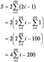
So the maximum sum is 2*(sum of odd numbers from 1 to 199). That is, the sum, S, is

The symbol is the Greek letter "Sigma". It stands for "Sum". So, stands for 1+2+...+100.

Recall from Algebra II that (1+2+3+ … + N) is calculated by the formula .

Therefore, .

In general, if n is the number of cases, we have two situations for computing the maximum possible sum:

n is even	n is odd

So, we can standardize our measures of association across different data sets (and hence different numbers of cases) by using the formula:

, where S is defined as above.

The value of A will always be between 0 and 1. The closer it is to 0, the more associated in the same direction is the ranked data. The data being near reverse order (as in above example) means A has a value near 1.

But two questions came up. First, does a value near 1 always imply that the two variables are in near reverse rank order (as in our example)? Second, what do values near .5 mean?

Beta pointed out that if you rearrange ranks on the same side of the "middle", then the sum of absolute differences does not change! So there could be MANY different ways that X and Y could produce 1 for the value of [sum(abs(rank(x)-rank(y))]/S, and those ways could range from X and Y being in perfect reverse rank order to each "half" being totally jumbled up.

Thus, this measure of association works well for high association in the same direction (meaning that when we know the measure has a value near 0 we can infer something definite about the relationship), but this measure doesn't work well when A is very much greater than 0. Too many dissimilar situations end up getting similar measures of association.

Whatever formula we might use, we would still face the same issue of wanting to use it to make comparisons across datasets of different sizes. In that regard, we could still use the same approach -- divide each measure of association by the maximum possible measure for that number of cases. But to do that, we must making sure that all the variables are on the same scale (as with Mary's approach of dividing each score by the variable's largest value -- making the possible values on every variable range from 0 to 1).

We could, for example, multiply standardized scores, as in . Here the values of X and Y are standardized by Mary’s technique of dividing each score by the variable’s largest value. To enable comparisons across data sets having different numbers of cases, you would need to standardize again, by dividing each sum by the largest possible value for that number of cases. Since the largest possible sum in this case would be gotten by each standardized score being 1, then the sum will be largest when every value is the same. This means that n is the maximum possible sum for two variables that are contain data on the same n cases. So,

will give a measure that you can use to compare across data sets. The measures will be "standardized" so that they take into account both how associated the variables are and different numbers of cases in the different pairs of variables. What we don't know is whether this measure is useful in distinguishing among strengths of associations. You will do that as an assignment.

Assignment: Investigate A₂ as a measure of association. Does it have drawbacks? Strengths? Does it work the way you think it ought to?

You already studied one method of putting all variables on the same scale -- converting them to z-scores. (Recall: You transform a set of scores into a set of z-scores by subtracting the set's mean score from each score and dividing each difference by the set's standard deviation).

We can define S₃ as . This is like S₂, except that we are standardizing the scores by changing them to z-scores instead of to percents. When we do this, it turns out that the sum has a maximum value of n-1. [Note 1]. So, if we define A₃ as , then A₃ will have a maximum value of 1 and a minimum value of -1. It will be 1 if every case has the same value on X as it does on Y. It will be -1 if every case has the opposite measure on X that it has on Y. It will be 0 if the scatterplot looks like a circle or square.

Assignment

1) Read pp. 111-119 in Basic Practice of Statistics

2) Go through ActivStats, Lesson 8 (Correlation)

3) Apply A₂ and A₃ as a measures of association. Use the Places Rating data. Are they consistent with the graphs? Can you predict what a scatterplot will look like (roughly) when given a specific value of A₂ or A₃?

Note 1. This is assuming that we have defined the variance as having a denominator of n-1. If we define the variance as having a denominator of n, then the sum is n.